1 Understanding Trees

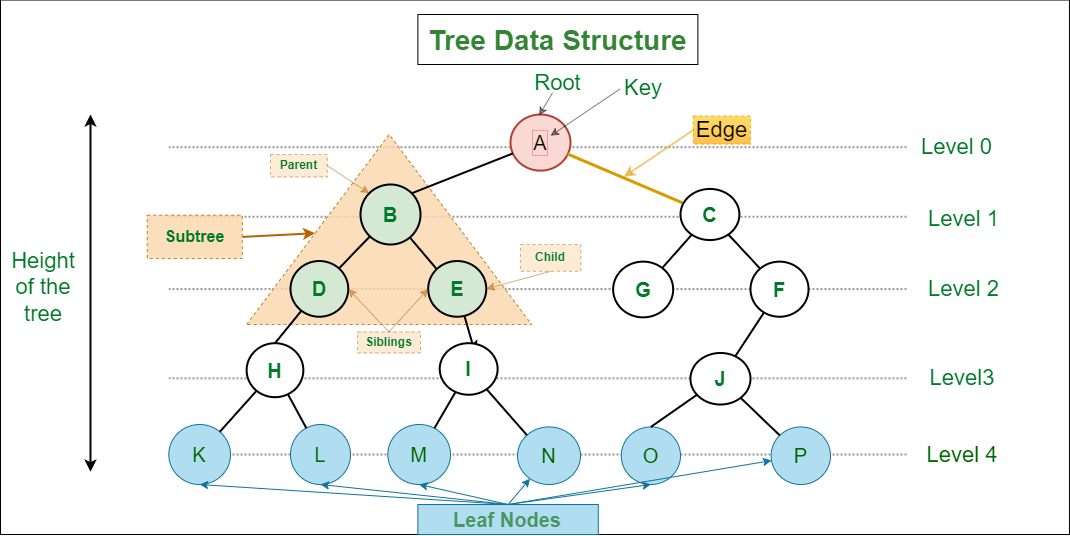
A tree is a hierarchical data structure composed of nodes connected by edges. Each node has a parent-child relationship, with a designated root node at the top. The nodes that do not have children are termed leaves. The node from which another node originates is the parent, and the node that stems from from a parent is a child.

2 Tree Terminologies

    A
   / \
  B   C
     / \
    D   E

Node:

• A node is an entity that contains a key or value and pointers to its child nodes.
• In this case, A, B, C, D, and E are nodes.
• The last nodes of each path are called leaf nodes or external nodes that do not contain a link/pointer to child nodes.
• The node having at least a child node is called an internal node.

Edge:

• It is the link between any two nodes.

Root:

• The topmost node in a tree. It is the starting point for traversing the tree and has no parent.
• A non-empty tree must contain exactly one root node.
• In the above example, A, is the root of the tree.

Parent:

• A node in a tree that has one or more child nodes. The node directly above a given node its parent.
• The node which is a predecessor of a node is called the parent node of that node.
• In the above example, A is the parent of B and C. C is the parent of D and E.

Child:

• A node in a tree that is directly connected to another node below it. Nodes with the same parent are called siblings.
• The node which is the immediate successor of a node is called the child node of that node.
• In the above example, B, D, and E are children of their respective parents.

Siblings:

• B and C are siblings, as are D and E.

Leaf (External Node):

• The nodes which do not have any child nodes are called leaf nodes.
• In the above example, B, D, and E are leaf nodes because they have no children.

Ancestor of a Node:

• Any predecessor nodes on the path of the root to that node are called Ancestors of that node. A and C are the ancestor nodes of the node D.

Internal Node:

• A, C, are internal nodes as they have at least one child.

Tree Path:

• Let's consider the path from node B to node E.

    A
   / \
  B   C
     / \
    D   E

• The path: B -> A -> C -> E

Tree Levels:

• The count of edges on the path from the root node to that node.
• The root node has level 0.

Each level represents a horizontal row of nodes:

Level 1: A
Level 2: B, C
Level 3: D, E

Node Degree:

• The degree of a node is the number of children it has. Most nodes in this example have a degree of 2, except for the leaf nodes (B, D, and E) with a degree of 0.

Height of a Node:

• The height of a node is the number of edges from the node to the deepest leaf (i.e., the longest path from the node to a leaf node).

Depth of a Node:

• The depth of a node is the number of edges from the root to the node.

Height of a Tree:

• The height of a tree is the length of the longest path from the root to a leaf:

Height of the tree: 2

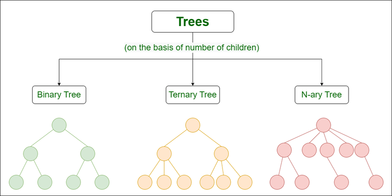
3 Types of Tree data structures(on the basis of number of children):

Based on the number of children each node can have, tree data structures can be categorized into various types.

1 Binary Tree:

In a binary tree, each node can have at most two children: a left child and a right child.

2 Ternary Tree:

A Ternary tree is a tree data structure in which each node has at most three child nodes, usually distinguished as left, mid, and right.

3 N-ary Tree:

A a N-ary tree, each node can have up to n children, where n is a fixed integer.

4 Types of Trees:

1. Binary Tress

Definition: A binary tree is a tree structure in which each node can have at most two children, typically referred to as the left child and the right child.

Key Characteristics:

• Nodes have, at most, two children.
• Efficient for search, and retrieval operations.

    A
   / \
  B   C
 / \
D   E

2. Binary Search Trees (BST):

Definition: A binary search tree is a specific type of binary tree where the left child is less than or equal to the parent, and the right child is greater.

Key Characteristics:

• Maintains sorted data for efficient searching.
• Allows for logarithmic time complexity for search operations.

    4
   / \
  2   6
 / \ / \
1  3 5  7

3. AVL Trees:

Definition: An AVL tree is a self-balancing binary search tree, ensuring that the heights of the two child subtrees of any node differ by at most one.

Key Characteristics:

• Guarantees logarithmic height, leading to efficient search, insertion, and deletion operations.

      3
     / \
    2   5
   /   / \
  1   4   6

4. B-Trees:

Definition: A B-tree is a self-balancing tree structure that maintains sorted data and is designed for use in database and file systems.

Key Characteristics:

• Nodes can have more than two children, providing efficient storage and retrieval for large datasets.

        3, 7
       / | \
      1  4  9
     / \    \
    0   2   10

5. Red-Black Trees:

Definition: A red-black tree is a type of self-balancing binary search tree where each node has an extra bit for denoting the color (red or black).

Key Characteristics:

• Ensures balanced trees, optimizing search, insertion and deletion operations.

      4 (B)
     / \
    2   6 (R)
   / \   \
  1   3   7

Representation of Trees

In C++, trees can be represented using various data structures. One of the most common representations is using a node-based approach, where each node represents an element of the tree, and pointers are used to connect nodes to form the hierarchical structure of the tree.

Node Structure:

First, we define a structure for the tree node. Each node contains a value and pointers to its children (if any).

#include <vector>

struct TreeNode {
    int data;
    std::vector<TreeNode*> children;

    TreeNode(int val) : data(val) {}
};

In this representation:

• TreeNode is a struct representing a node in the tree.
• It contains an int member named data to store the value of the node.
• children is a vector of pointers to other TreeNode objects, representing the children of the node.

Now, let's create a simple tree using this representation:

int main() {
    // Creating nodes
    TreeNode* root = new TreeNode(1);
    TreeNode* child1 = new TreeNode(2);
    TreeNode* child2 = new TreeNode(3);

    // Connecting nodes
    root->children.push_back(child1);
    root->children.push_back(child2);

    // Adding children to child1
    TreeNode* child11 = new TreeNode(4);
    TreeNode* child12 = new TreeNode(5);
    child1->children.push_back(child11);
    child1->children.push_back(child12);

    // Adding a child to child2
    TreeNode* child21 = new TreeNode(6);
    child2->children.push_back(child21);

    // Clean up memory (not necessary in this example but good practice)
    delete root;
    delete child1;
    delete child2;
    delete child11;
    delete child12;
    delete child21;

    return 0;
}

This code creates a tree with the following structure:

    1
   / \
  2   3
 / \   \
4   5   6