
Memory
Memory, in the context of computers, refers to the hardware devices used to store data and instructions temporarily or permanently for immediate use in a computer or other digital electronic device. It is essential for storing and retrieving data and instructions that the CPU (central processing unit) needs to execute tasks.
Computer memory can be broadly categorized into two types:
- Primary Memory (Main Memory): This type of memory is directly accessible by the CPU and is used to store data and instructions that are currently being executed or manipulated. It is volatile, meaning its contents are lost when the computer is powered off. Examples include RAM (Random Access Memory).
- Secondary Memory (Storage): This type of memory is used for long-term storage of data and instructions. It is non-volatile, meaning its contents are retained even when the power is turned off. Examples include hard drives, solid-state drives (SSDs), and optical disks.
What is Stack Memory?
Stack memory is a region of memory used for temporary storage during the execution of programs. It holds:
- Function call information (return addresses, parameters).
- Local variables for functions.
- Control flow information (like saved registers).
It is called the "stack" because data is added and removed in a Last-In-First-Out (LIFO) manner. Every time a function is called, a block of memory (called a stack frame) is added to the top of the stack, and when the function returns, this block is removed.
How Stack Memory Works
When a function is called:
- A stack frame is created and pushed onto the stack. This stack frame contains:
- The return address (the point in the code where the function will return after execution).
- Function parameters.
- Local variables used by the function.
- The saved frame pointer (if used) and the state of some registers.
When a function finishes:
- The stack frame is popped off the stack, and the program resumes from the return address, restoring the previous state.
Stack Frame Layout
A typical stack frame contains the following elements:
- Return Address: This stores the address of the instruction where the program should return after the function call completes.
- Parameters: Arguments passed to the function, either via registers or directly on the stack.
- Saved Frame Pointer (Base Pointer or Frame Pointer): If the architecture uses frame pointers (like
ebpin x86), the previous frame pointer is saved to allow access to local variables and parameters. - Local Variables: Variables that are declared within the function. These are typically placed on the stack and are automatically cleaned up when the function ends.
- Saved Registers: Some architectures require the saving of certain CPU registers before calling another function.
Stack layout during function call:
+---------------------------+
| Parameters (if any)        |  <-- Passed arguments
+---------------------------+
| Return address             |  <-- Address to return to
+---------------------------+
| Old base pointer (EBP)     |  <-- Old base pointer
+---------------------------+
| Local variables            |  <-- Function's local data
+---------------------------+
| (Stack grows downward)     |
Characteristics of Stack Memory
- LIFO (Last-In-First-Out) Nature: The stack grows when a function is called (pushing stack frames), and shrinks when a function returns (popping stack frames).
- Size Limitations: The size of the stack is typically fixed and small compared to the heap (e.g., a few MBs). If a program uses too much stack memory (e.g., deep recursion or large local variables), it can cause a stack overflow.
- Automatic Memory Management: Stack memory is automatically allocated and deallocated. When a function is called, its stack frame is allocated; when the function returns, the frame is deallocated. The programmer doesn’t need to explicitly free the memory.
- It does not require explicit intervention from the programmer.
- Fast Access: Since the stack memory operates in a very controlled and structured manner (LIFO), it is fast to allocate and deallocate compared to heap memory.
- Function Scope: Variables stored in the stack are local to the function and are only valid while the function is running. Once the function exits, these variables are destroyed.
Stack Overflow
Stack overflow occurs when a program tries to use more stack memory than is available. Common causes include:
- Deep recursion: Each recursive call adds a new stack frame, and if the recursion depth is too large, the stack runs out of space.
- Large local variables: Declaring large arrays or data structures as local variables can quickly exhaust stack space.
void recursive_function() {
    recursive_function();  // Recursive call without base case
}

int main() {
    recursive_function();  // This will cause a stack overflow
    return 0;
}
Stack Memory in Multi-Threading
In multi-threaded environments, each thread gets its own stack. The size of a thread’s stack is typically smaller than the main thread’s stack and is limited by system settings. This is why recursive functions or large local variables in threads are more prone to stack overflow.
Thread Stack:
- Each thread's stack is separate from others, and each thread operates with its own stack space.
- If a thread exhausts its stack space (for example, due to recursion), it can cause a stack overflow for that particular thread without affecting other threads.
Stack Memory in Different Architectures
a. x86 (32-bit architecture):
In 32-bit x86 architecture, the stack grows downward (from high memory to low memory). The stack pointer register (esp) tracks the top of the stack, and the base pointer register (ebp) is used to reference local variables and function parameters.
b. x86_64 (64-bit architecture):
In 64-bit systems, the stack works similarly, but with 64-bit registers like rsp (stack pointer) and rbp (base pointer). Function parameters are often passed through registers (rdi, rsi, etc.), with the stack holding additional parameters and local variables.
c. ARM architecture:
In ARM, the stack grows downward as well. The stack pointer (sp) is used to point to the top of the stack. ARM typically uses a link register (LR) to store the return address, which helps in reducing stack usage for return addresses.
Example Code Using Stack Memory (C)
void functionA(int a) {
    int b = 20;  // Local variable stored on the stack
    printf("Value of a: %d, Value of b: %d\n", a, b);
}

int main() {
    int x = 10;  // Local variable stored on the stack
    functionA(x);  // Function call, new stack frame created
    return 0;
}
In this example:
- When
main()is called, a stack frame is created formain(), containingx. - When
functionA()is called, a new stack frame is pushed, containingaandb. - When
functionA()returns, its stack frame is popped, and the program continues frommain().
Function Calls and Stack Frames
When a function is called, the compiler generates the necessary instructions to create a new stack frame. This frame includes:
- The return address (so the program knows where to return after the function finishes).
- Function parameters.
- Local variables.
- Saved registers (if required).
- In some cases, the frame pointer to help with accessing variables in the current stack frame.
- When the function returns, the compiler generates instructions to clean up the stack frame, which involves restoring the return address and freeing the space used by the local variables.
Stack Frame Creation (Prologue)
- The prologue of a function (generated by the compiler) sets up the stack frame:
- Save the return address: The address of the instruction after the function call is pushed onto the stack.
- Save the previous frame pointer (if used): The current frame pointer is saved to the stack to preserve the calling function’s frame.
- Allocate space for local variables: The stack pointer is adjusted to make room for local variables.
Example (in x86 assembly):
push ebp          ; Save the old base pointer
mov ebp, esp      ; Set the new base pointer
sub esp, <size>   ; Allocate space for local variables
Stack Frame Cleanup (Epilogue)
- The epilogue of a function is responsible for cleaning up the stack:
- Restore the frame pointer: If a frame pointer was used, it is restored to the previous value.
- Pop the return address: The return address is popped from the stack, and the program continues execution from that address.
Example (in x86 assembly):
mov esp, ebp      ; Restore the stack pointer
pop ebp           ; Restore the old base pointer
ret               ; Return to the caller (pop the return address)
Inline Functions and Optimization
- Modern compilers also optimize stack usage. For example, inline functions (which are small functions that the compiler replaces with the actual code instead of creating a function call) don’t use the stack at all. The function code is directly substituted into the caller’s code, avoiding stack frame creation.
Pros and Cons of Stack Memory
Pros of Stack Memory:
- Fast Memory Allocation and Deallocation:
- Pro: Stack memory is allocated and deallocated in a predictable, efficient manner using a Last-In-First-Out (LIFO) structure. Since the stack operates in this controlled way, memory allocation and deallocation are extremely fast compared to the heap, where memory is dynamically allocated.
- Reason: The stack simply moves the stack pointer up or down, requiring minimal instructions.
- Automatic Memory Management:
- Pro: The stack is automatically managed by the compiler. The programmer does not need to worry about manually allocating or freeing memory for local variables and function call information. When a function call is made, its stack frame is automatically created, and when it finishes, the frame is destroyed.
- Reason: Each function call pushes a new frame onto the stack, and returning from a function pops it off, making it easy to track memory usage for local variables.
- No Memory Fragmentation:
- Pro: Unlike heap memory, which can become fragmented over time due to dynamic allocation and deallocation, the stack doesn't suffer from fragmentation. The stack pointer moves up and down in a contiguous memory block, keeping memory tightly packed.
- Reason: The LIFO nature of the stack means memory is always allocated and deallocated in an orderly fashion.
- Locality of Reference:
- Pro: Stack memory is often accessed in a predictable manner, making it more likely to benefit from cache locality. Since the stack is used frequently for storing function call information and local variables, it is often stored in the faster cache memory close to the CPU.
- Reason: The spatial and temporal locality of stack data ensures it can be quickly accessed.
- Predictable Lifetime of Variables:
- Pro: Variables in the stack have a well-defined lifetime. They are created when the function is called and destroyed when the function returns. This makes the stack ideal for local variables whose scope is limited to the function in which they are declared.
- Reason: As soon as a function exits, its stack frame is popped, and all its local variables are deallocated.
- Simple to Implement:
- Pro: Stack memory is straightforward to manage from a systems programming perspective. The structure and behavior are fixed, making it easy to implement in hardware and software.
- Reason: Its LIFO behavior simplifies both allocation and deallocation logic, reducing complexity compared to more complex memory models like the heap.
Cons of Stack Memory:
- Limited Size:
- Con: The size of the stack is typically much smaller than heap memory. The stack has a fixed size (usually defined by the operating system), and it is easy to run out of stack space, especially with deep recursion or large local variables.
- Reason: Operating systems often impose strict limits on stack size (e.g., a few MB), which can lead to stack overflow if the limit is exceeded.
- Stack Overflow:
- Con: Since the stack has a fixed size, it is possible to exhaust available stack space, causing a stack overflow. This is particularly common with recursive function calls that do not have a base case, or when large local variables are declared.
- Reason: The LIFO structure means once the stack reaches its size limit, it can’t grow further. Any attempt to push more data onto the stack results in a stack overflow.
- Not Suitable for Large Dynamic Data:
- Con: The stack is not ideal for dynamically-sized or large data structures, such as large arrays, linked lists, or trees. These types of data are better managed in the heap because the stack is limited in both size and flexibility.
- Reason: Large data structures can quickly exhaust stack space, whereas the heap can dynamically allocate memory as needed.
- Short Lifetime for Variables:
- Con: Variables stored in stack memory are automatically destroyed when the function call completes. This makes it difficult to retain data across function calls unless the data is passed explicitly or stored elsewhere (like the heap).
- Reason: Stack memory is tied to the scope of a function, meaning variables are destroyed once the function exits.
- No Flexibility for Memory Reuse:
- Con: The stack's LIFO nature means memory can only be reused when the stack unwinds. This lack of flexibility makes the stack unsuitable for general-purpose dynamic memory management, unlike the heap, which allows for arbitrary allocation and deallocation at any time.
- Reason: The LIFO model ensures that only the most recently allocated memory can be freed.
- No Explicit Control Over Memory Allocation:
- Con: Stack memory is allocated and freed automatically, so the programmer has no explicit control over its management. While this is often an advantage, it can be a drawback in situations where finer control over memory allocation is needed (e.g., for long-term data storage).
- Reason: The stack is automatically managed, meaning developers cannot directly control when or how memory is freed beyond ensuring that functions return properly.
- Limited to Local Variables and Function Calls:
- Con: Stack memory is restricted to storing local variables and function call information. It cannot be used for globally persistent data or complex data structures that require long-term memory management.
- Reason: Since the stack is bound to the lifetime of function calls, it is unsuitable for data that needs to persist across different parts of the program.
Allocator
1️⃣ Linear | Bump Allocator
The linear allocator (also called the bump allocator) is one of the simplest forms of memory allocation used in OS development. It allocates memory in a contiguous, linear fashion, making it extremely fast with minimal overhead.
Components:
- Memory Block
- It consists of a block of memory.
- Pointer
- It points to the beginning of the designated memory block.
Mechanism:
Memory Allocation: When memory is requested, the allocator moves the pointer forward by the size of the requested memory. This is called bumping the pointer.
No Deallocation: Memory allocated cannot be freed individually. The only way to reclaim memory is to reset the pointer back to the starting position of the memory block.
Example Code:
#define MEMORY_SIZE 1024  // Define the size of the memory block

char memory[MEMORY_SIZE]; // Create a fixed-size memory block
char* bump_pointer = memory; // Initialize the bump pointer

void* bump_allocate(size_t size) {
    // Check if enough space is available
    if (bump_pointer + size > memory + MEMORY_SIZE) {
        return NULL; // Out of memory
    }

    void* allocated_memory = bump_pointer; // Allocate memory
    bump_pointer += size; // Bump the pointer forward
    return allocated_memory; // Return the allocated address
}

void bump_reset() {
    bump_pointer = memory; // Reset the bump pointer to the start
}
Advantages
- Speed: Allocation is fast since it involves only pointer arithmetic.
- Simplicity: The implementation is straightforward, requiring minimal bookkeeping.
- Low Overhead: No metadata is required for each allocation, which saves memory.
Disadvantages
- No Fine-Grained Control: You cannot free individual allocations; memory can only be reclaimed in bulk by resetting the pointer.
- Memory Waste: If a large block of memory is allocated and not fully used, it can lead to waste.
- Fragmentation: In long-running programs, if the allocator is used repeatedly and then reset, it can lead to fragmentation if memory usage patterns are not predictable.
2️⃣ Arena Allocator
An arena allocator (region-based) organizes memory into multiple regions (or arenas). Each arena can manage its own allocations independently, allowing for faster allocation and deallocation processes without affecting other arenas. This technique helps to reduce fragmentation and manage memory more effectively in complex applications.
Mechanism:
- Memory Pool Creation: A large block of memory is divided into smaller, fixed-size arenas. Each arena can be allocated independently.
- Pointer Initialization: Each arena has its own pointer (often referred to as the "arena pointer") that tracks the current position for allocations.
- Memory Allocation:
- When a request for memory is made, the allocator checks the current arena's pointer to see if enough space is available.
- If sufficient space exists, memory is allocated, and the arena pointer is incremented by the size of the allocated memory.
- If the arena is full, a new arena can be created, or a suitable arena can be chosen based on the allocation request.
- Memory Deallocation:
- Memory can be deallocated on an arena-by-arena basis.
- When an arena is no longer needed, it can be freed entirely, reclaiming all its memory at once.
- Individual allocations within an arena can also be managed, though it typically involves some form of bookkeeping.
Example:
#include <stdlib.h>
#include <stdio.h>

#define ARENA_SIZE 1024 // Define the size of each arena

typedef struct Arena {
    char memory[ARENA_SIZE]; // Memory block for the arena
    size_t offset;           // Current offset for allocation
    struct Arena* next;      // Pointer to the next arena
} Arena;

// Function to create a new arena
Arena* create_arena() {
    Arena* arena = (Arena*)malloc(sizeof(Arena));
    if (arena) {
        arena->offset = 0;
        arena->next = NULL;
    }
    return arena;
}

// Function to allocate memory from a specific arena
void* arena_allocate(Arena* arena, size_t size) {
    // Check if enough space is available
    if (arena->offset + size > ARENA_SIZE) {
        return NULL; // Out of memory in this arena
    }

    void* allocated_memory = &arena->memory[arena->offset]; // Allocate memory
    arena->offset += size; // Move the offset forward
    return allocated_memory; // Return the allocated address
}

// Function to free an entire arena
void free_arena(Arena* arena) {
    free(arena); // Free the entire arena
}

// Function to demonstrate multiple arenas in use
void demo_multiple_arenas() {
    Arena* arena1 = create_arena();
    Arena* arena2 = create_arena();
    Arena* arena3 = create_arena();

    if (!arena1 || !arena2 || !arena3) {
        perror("Failed to create arenas");
        return;
    }

    // Allocate from Arena 1
    int* num1 = (int*)arena_allocate(arena1, sizeof(int));
    if (num1) {
        *num1 = 42;
        printf("Arena 1 allocated number: %d\n", *num1);
    }

    // Allocate from Arena 2
    char* str1 = (char*)arena_allocate(arena2, 20 * sizeof(char));
    if (str1) {
        snprintf(str1, 20, "Hello, Arena 2!");
        printf("Arena 2 allocated string: %s\n", str1);
    }

    // Allocate from Arena 3
    double* num2 = (double*)arena_allocate(arena3, sizeof(double));
    if (num2) {
        *num2 = 3.14;
        printf("Arena 3 allocated number: %.2f\n", *num2);
    }

    // Free all arenas
    free_arena(arena1);
    free_arena(arena2);
    free_arena(arena3);
}

int main() {
    demo_multiple_arenas(); // Demonstrate the use of multiple arenas
    return 0;
}
Advantages:
- Reduced Fragmentation: Since each arena manages its own allocations, the risk of fragmentation is minimized, making memory management more efficient.
- Faster Allocations: Allocating memory from an arena can be quicker than traditional allocation methods because it involves simple pointer arithmetic.
- Batch Deallocation: Freeing an entire arena can reclaim a large amount of memory in one operation, which is often faster than freeing individual allocations.
- Flexibility: Allows for multiple allocation strategies (e.g., different sized arenas for different usage patterns).
Disadvantages:
- Memory Waste: If an arena is created but not fully utilized, the unused memory within that arena can lead to waste.
- Complex Implementation: Compared to simpler allocators, implementing an arena allocator can be more complex, particularly when managing multiple arenas and their lifetimes.
- Overhead: Each arena requires a small amount of overhead for bookkeeping, which may be significant if many small arenas are created.
Memory Address Space
Memory address space refers to the range of addresses that a processor or device can use to access memory. It is a conceptual model that represents all possible addresses in a system’s memory that a processor can refer to for reading or writing data. Each address in the memory space corresponds to a byte, word, or another data unit depending on the system architecture.
Types of Memory Address Space
1️⃣ Physical Address Space
The address space the CPU exposes to the hardware.
The actual hardware memory, such as RAM (Random Access Memory), that is installed on the system. Each address here corresponds to a location in the physical memory hardware.
The size of the physical address space depends on the number of address lines supported by the processor. For example, a 32-bit processor can address up to 4 GB of physical memory, while a 64-bit processor can theoretically address up to 16 exabytes (though actual systems are usually limited to much less due to practical hardware constraints).
2️⃣ Virtual Address Space | Logical Address Space
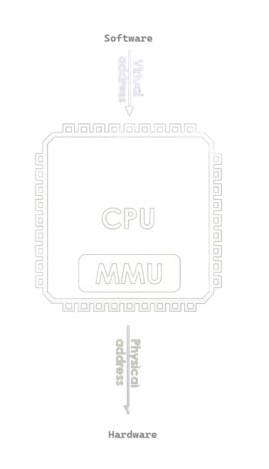
The address space the CPU exposes to the software.
- This is an abstraction used by operating systems to provide each process with its own private address space, independent of other processes. The operating system maps virtual addresses to physical memory locations using page tables and memory management units (MMUs).
- Each process sees its own memory starting from address 0, even though the actual data is mapped to different physical addresses.
Difference Between Logical and Physical Address Spaces
- Logical (Virtual) Address Space:
- Generated by the CPU during program execution.
- Mapped to physical addresses using paging or segmentation.
- Larger than physical memory, enabling the use of virtual memory.
- Physical Address Space:
- Refers to the actual addresses in RAM.
- Physical memory is finite and smaller than logical address space.
Address Space Translation
Address space translation is the process of converting logical (virtual) addresses to physical addresses. This is typically done by the Memory Management Unit (MMU), a hardware component in the CPU. The MMU uses tables, such as page tables or segment tables, to perform this mapping.
- Page Table: A table used in paging that holds the mapping between a process's virtual pages and the physical frames in RAM.
- Segment Table: Used in systems that employ segmentation. It maps the segment number in the virtual address to the base address in physical memory.
Memory Translation Systems
Memory translation systems are the mechanisms used by computer systems to translate logical (or virtual) addresses generated by programs into physical addresses that correspond to actual locations in physical memory (RAM). This translation is essential in systems that use virtual memory and allows processes to operate as if they have access to a large, contiguous block of memory, even when physical memory is smaller or fragmented.
The most common memory translation systems are paging, segmentation, and hybrid approaches that combine both. These systems rely on hardware support, typically via the Memory Management Unit (MMU), to perform the necessary translations efficiently.
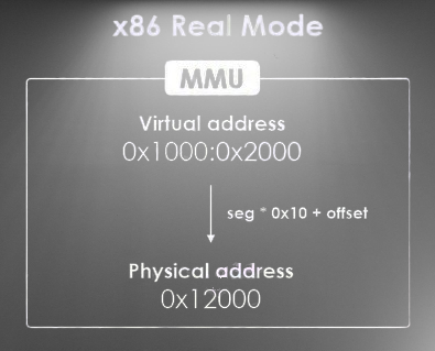
1 Segmentation
Segmentation divides memory into variable-sized segments that correspond to logical divisions of a program, such as code, data, stack, etc. Each segment is independent and has its own base address and limit, providing a more logical division of memory than paging.
How Segmentation Works:
- The logical address space is divided into segments, each of which may be of a different size.
- Each segment has a base address (starting point in physical memory) and a limit (the length of the segment).
- The segment table keeps track of the base and limit of each segment.
When a program accesses memory:
- The logical address consists of a segment number and an offset within that segment.
- The MMU looks up the base address of the segment from the segment table and adds the offset to calculate the physical address.
Example of Segmentation:
- If a program accesses memory using the logical address
(segment 3, offset 0x100), the MMU will look up segment 3 in the segment table, retrieve the base address (e.g.,0x2000), and add the offset0x100to produce the physical address0x2100.
Advantages of Segmentation:
- Logical division of programs: Segments correspond to logical units (e.g., code, data), making it easy to protect and share memory between processes.
- Supports dynamic memory growth: Segments can grow or shrink dynamically, unlike fixed-sized pages in paging.
Disadvantages of Segmentation:
- External fragmentation: Since segments can be of varying sizes, free memory can become fragmented.
- More complex memory management: Managing segments of varying sizes requires more effort than fixed-size pages.
Address Translation in Segmentation:
- A logical address is divided into:
- Segment number: Used to look up the base address of the segment in the segment table.
- Offset: The offset within the segment is added to the base address to get the physical address.
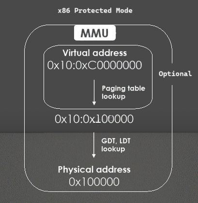
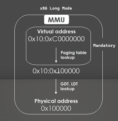
2 Paging
Paging is one of the most widely used memory translation systems in modern computers. It breaks both the virtual address space and physical memory into fixed-size blocks called pages (for virtual addresses) and frames (for physical memory).
- On x86_* architectures this is achieved via hardware.
How Paging Works:
- The logical address space is divided into fixed-size pages (e.g., 4 KB or 8 KB).
- The physical address space is divided into the same-sized fixed blocks called frames.
- A page table is maintained by the operating system for each process, which keeps track of the mapping between the virtual pages and the corresponding physical frames.
When a program accesses memory:
- The virtual page number from the logical address is used as an index into the page table.
- The page table provides the frame number, and this is combined with the offset within the page to produce the final physical address.
- The MMU handles the translation of virtual addresses to physical addresses based on the page table entries.
Example of Paging:
- Suppose a virtual address
0x12345needs to be translated to a physical address. - The system divides this address into a page number (e.g.,
0x12) and an offset within that page (e.g.,0x345). - The MMU looks up the page table to find out which physical frame is associated with page
0x12and combines it with the offset0x345to produce the physical address.
Advantages of Paging:
- No external fragmentation: Memory is allocated in fixed-sized pages, so no gaps of unusable memory are created.
- Efficient use of memory: Pages are allocated dynamically, and programs only use the memory they need at any time.
Disadvantages of Paging:
- Internal fragmentation: A program may not use the entire page, resulting in some wasted space.
- Page table overhead: Maintaining large page tables (especially in systems with large address spaces) can be memory- and time-consuming.
Address Translation in Paging:
- A logical address is divided into:
- Page number: Used to index into the page table to find the corresponding frame.
- Offset: The offset within the page remains unchanged and is added to the base address of the frame.
Memory Management Techniques
Memory management techniques are methods used to efficiently allocate, track, and manage the memory of a computer system. These techniques ensure optimal use of available memory while preventing issues such as fragmentation, memory leaks, and inefficient usage. Below are the key memory management techniques:
1️⃣ Contiguous Memory Allocation
It is one of the simplest memory management techniques. In this process, each process is allocated a single contiguous block of memory. This allocation scheme ensures that each process' memory be assigned to consecutive physical address. It ensures that the entire program is stored in one single contiguous area of memory.
Types of Contiguous Memory Allocation:
- Fixed Partitioning (Static Allocation):
- The memory is divided into fixed-size partitions during system initialization.
- Each partition can hold exactly one process.
- Internal Fragmentation occurs when a process doesn't fully utilize its allocated partition, resulting in wasted space inside that partition.
- Variable Partitioning (Dynamic Allocation):
- Partitions are created dynamically based on the size of the process requesting memory.
- Each process is allocated exactly the amount of memory it needs.
- External Fragmentation occurs when free memory becomes scattered and cannot be used efficiently by new processes, even though enough total memory may be available.
Scenario:
Suppose a system has 1000 KB of memory, and processes A, B, C, and D need to be allocated space in this memory. The system uses contiguous memory allocation, meaning each process must be allocated in a single, continuous block of memory. Let's assume:
- Process A requires 200 KB
- Process B requires 300 KB
- Process C requires 100 KB
- Process D requires 250 KB
Initial Allocation:
The memory is allocated in order as follows:
- Process A is allocated the first 200 KB (Memory 0-199 KB)
- Process B is allocated the next 300 KB (Memory 200-499 KB)
- Process C is allocated the next 100 KB (Memory 500-599 KB)
- Process D is allocated the next 250 KB (Memory 600-849 KB)
At this point, there is 150 KB of free memory left (Memory 850-999 KB), which is not enough to accommodate a new process that requires more than 150 KB.
Process B Terminates:
Now, let's say Process B terminates and releases its allocated 300 KB of memory (Memory 200-499 KB). The memory layout looks like this:
| 0-199 KB | 200-499 KB | 500-599 KB | 600-849 KB | 850-999 KB |
|---|---|---|---|---|
| Process A | Free | Process C | Process D | Free |
So, there are now two free blocks of memory:
- 300 KB (from Process B)
- 150 KB (remaining at the end)
New Process E Arrives:
Now, suppose Process E needs 350 KB of memory. Even though there is 450 KB of total free memory available, it is fragmented into two separate blocks (300 KB and 150 KB). Contiguous memory allocation requires that Process E be allocated in one continuous block of 350 KB, but neither of the two free blocks is large enough. This fragmentation is known as the external fragmentation.
Memory Compaction:
It involves dynamic relocation.
To accommodate Process E, the system may perform memory compaction. This involves shifting processes C and D up in memory to create one large free block. After compaction, the memory layout looks like this:
| 0-199 KB | 200-299 KB | 300-549 KB | 550-999 KB |
|---|---|---|---|
| Process A | Process C | Process D | Free |
Now, there is 450 KB of contiguous free memory (550-999 KB), which is enough to allocate the 350 KB required by Process E. The final memory layout would be:
| 0-199 KB | 200-299 KB | 300-549 KB | 550-899 KB | 900-999 KB |
|---|---|---|---|---|
| Process A | Process C | Process D | Process E | Free |
Solution of External Fragmentation:
External fragmentation occurs when free memory is available, but it is fragmented into small, non-contiguous blocks. As a result, even though there is enough total free memory to satisfy a process's request, the process cannot be allocated memory because the free blocks are too small or scattered.
🅰️ Compaction:
It is technique in which the operating system periodically moves processes in memory to consolidate all free memory into a single large contiguous block.
- How It Works:
- The system shifts processes so that they are placed next to each other, eliminating gaps between them.
- All free memory is then placed in one contiguous block at the end of memory.
- Advantages:
- Eliminates external fragmentation by creating a large, contiguous free block.
- Allows larger processes to be accommodated in memory.
- Disadvantages:
- High overhead: Compaction is computationally expensive because it involves moving memory contents during program execution.
- Requires dynamic relocation: Systems need to have relocation mechanisms (like base and limit registers) to adjust memory addresses during compaction.
- Time Consuming: Compaction can be expensive in terms of performance because processes need to be paused and moved, which involves copying large amounts of data in memory.
- Use Cases: Best suited for systems with infrequent memory allocation or systems that can tolerate delays during compaction.
🅱️ Paging:
Paging is a memory management technique that eliminates external fragmentation by dividing memory into fixed-size blocks called pages (in logical memory) and frames (in physical memory). Pages from processes are loaded into available frames in physical memory, which can be non-contiguous.
2️⃣ Non-Contiguous Memory Allocation
Non-contiguous memory allocation is a memory management scheme that allows processes to be allocated memory in different locations in physical memory, rather than requiring a single contiguous block. This approach helps overcome the limitations of contiguous memory allocation, particularly external fragmentation and inefficient use of memory.
There are two fundamental approaches to implement non-contiguous memory allocation.
🅰️ Paging:
In traditional memory allocation, processes are assigned a large, continuous block of memory, leading to problems such as external fragmentation (small gaps of unused memory) and the need for compaction to create larger free blocks.
Paging divides the logical (or virtual) memory of a process into fixed-size blocks (units) called pages, and the physical memory into blocks of the same size called frames. Pages in logical memory can be mapped to any available frame in physical memory, allowing processes to use scattered blocks of memory without needing a contiguous block.
Basic Concepts of Paging:
- Page: A fixed-size block of virtual memory (e.g., 4 KB).
- Frame: A fixed-size block of physical memory (e.g., 4 KB).
- A page is mapped to a frame, so the page number translates to a frame number in the physical memory.
Both pages and frames are of the same size (e.g., 4 KB). A process’s virtual address space is divided into pages, and these pages are loaded into available frames in the physical memory.
The logical address space of a process is divided into pages, while the physical memory is divided into frames. Pages from a process are stored in available frames of the physical memory, and these frames do not need to be contiguous.
Page Table:
- Each process has its own page table, which stores the mapping between the process's virtual pages and the physical frames. The operating system uses this table to translate virtual addresses into physical addresses during program execution.
Address Translation:
- When a process references a memory location, it provides a virtual address. This virtual address is divided into two parts:
- Page number (p): Identifies the page in the virtual address space.
- Offset (d): Specifies the exact location within that page.
The page number is used to look up the frame number in the page table, and the offset is used to find the exact byte within the frame. This process converts the virtual address into a physical address.
Example of Address Translation:
Consider a process with a virtual address space of 16 KB, divided into 4 pages (each 4 KB). If the process generates a virtual address 0x1234:
- Page Number (p): The first few bits of the address, identifying which page.
- Offset (d): The rest of the bits, identifying the byte within the page.
Let’s assume the page table maps Page 1 to Frame 5. The operating system will replace the page number with the frame number and add the offset to find the exact physical address.
🅱️ Segmentation:
Segmentation is a memory management scheme that divides a program's memory into variable-sized segments based on logical divisions, such as functions, data structures, or modules. Unlike paging, which divides memory into fixed-size blocks, segmentation reflects the program's logical structure, where each segment can grow or shrink independently, making it more flexible but also prone to fragmentation.
Key Concepts of Segmentation:
Segments:
- A segment is a logical division of a program's memory space. Each segment represents a meaningful part of the program, such as:
- Code segment (instructions of the program)
- Data segment (global variables)
- Stack segment (for function calls and local variables)
- Heap segment (for dynamically allocated memory)
Each segment has a segment number and a segment size. Unlike paging, segments are variable in size.
- A segment is a logical division of a program's memory space. Each segment represents a meaningful part of the program, such as:
Segment Table:
- Each process has its own segment table, which stores information about each segment:
- Base address: The starting address of the segment in physical memory.
- Limit: The length (or size) of the segment.
The segment table is used by the operating system to map a segment's logical address to the physical address in memory.
- Each process has its own segment table, which stores information about each segment:
- Logical Address in Segmentation:
- A logical address in segmentation consists of two parts:
- Segment number: Identifies the specific segment (e.g., segment 0 could be the code segment).
- Offset: The distance from the start of the segment to the exact memory location being accessed.
- A logical address in segmentation consists of two parts:
Example:
Suppose a program has three segments:
- Segment 0: Code (length 2000 bytes)
- Segment 1: Data (length 500 bytes)
- Segment 2: Stack (length 300 bytes)
A logical address might be (Segment 1, Offset 100):
- The segment number is 1 (data segment).
- The offset is 100 bytes within the data segment.
- The segment table would provide the base address for segment 1. If the base address is 5000, the physical address would be
5000 + 100 = 5100.
Memory Allocation Strategies
1️⃣ First Fit
- The First Fit strategy allocates the first available free block of memory that is large enough to satisfy a process’s memory request. The memory manager scans the list of free memory blocks from the beginning and selects the first one that fits.
Example:
- Available memory blocks: 10 MB, 5 MB, 15 MB, 20 MB.
- If a process requests 12 MB, the system will skip the 10 MB block and allocate the 15 MB block, leaving 3 MB free.
Pros:
- Fast allocation: It scans the list of memory blocks and stops at the first suitable block, reducing search time.
- Simple to implement.
Cons:
- Can lead to external fragmentation: Small leftover free blocks accumulate in memory, making it harder to allocate memory for larger processes.
2️⃣ Best Fit
- The Best Fit strategy allocates the smallest free block of memory that is large enough to satisfy the process’s request. The system scans the entire list of free blocks and selects the block that leaves the least amount of wasted space.
Example:
- Available memory blocks: 10 MB, 5 MB, 15 MB, 20 MB.
- If a process requests 12 MB, the 15 MB block will be chosen (leaving 3 MB free), because it is the smallest block that can accommodate the process.
Pros:
- Minimizes internal fragmentation: Because it picks the smallest possible block, there is less wasted memory within the allocated block.
Cons:
- Slower allocation: The entire list of free blocks must be scanned, which can take longer.
- Can lead to external fragmentation: Small leftover blocks can still result in fragmentation, even if it’s minimized.
3️⃣ Worst Fit
- The Worst Fit strategy allocates the largest free block of memory. This strategy aims to leave the largest remaining free block after allocation, under the assumption that larger blocks are more useful for future allocations.
Example:
- Available memory blocks: 10 MB, 5 MB, 15 MB, 20 MB.
- If a process requests 12 MB, the system will allocate the 20 MB block (leaving 8 MB free).
Pros:
- Reduces small fragmentation: By allocating the largest block, it tries to leave usable blocks of free memory after allocation.
Cons:
- Can waste large blocks: It can lead to underutilization of large memory blocks, leaving them unusable for smaller processes.
- Slower allocation: Like Best Fit, Worst Fit requires scanning the entire list of free blocks, which can slow down allocation.
4️⃣ Next Fit
- Next Fit is a variation of the First Fit strategy. Instead of starting the search for free memory from the beginning each time, the system starts from the location of the last allocation. This reduces search time for memory allocation.
Example:
- Available memory blocks: 10 MB, 5 MB, 15 MB, 20 MB.
- If a process was last allocated from the 10 MB block and the next process requests 12 MB, the system starts scanning from the 5 MB block.
Pros:
- Faster than First Fit: Since the system doesn’t always start scanning from the beginning, it reduces the overall search time.
Cons:
- Fragmentation: Like First Fit, Next Fit can also lead to external fragmentation due to scattered small blocks of free memory.
Knowledge Center
Fragmentation:
🅰️ External Fragmentation
Occurs when there is enough free memory in total, but it is not contiguous. Small free blocks of memory scattered throughout the system prevent larger processes from being allocated memory, even though the total free memory is sufficient.
🅱️ Internal Fragmentation
Occurs when the allocated memory block is larger than what the process actually needs. This results in some unused memory within the allocated block.

Leave a comment
Your email address will not be published. Required fields are marked *