1 Anatomy of a Binary Tree:

A binary tree is composed of nodes, where each node can have at most two children: a left child and a right child. The topmost node is called the root, and nodes without children are termed leaves. Nodes with a common parent are referred to as siblings.

The topmost node in a binary tree is called the root. Each node in a binary tree can have zero, one, or two children. If a node has no children, it is called a leaf node.

• The binary tree's structure allows for efficient searching and manipulation of data.

Consider the following binary tree as an example:

        A
       / \
      B   C
     / \
    D   E

In this tree, A is the root, B and C are its children, and D and E are children of B. D and E are leaf nodes as they have no children.

2 Key Properties

Binary Tree Degree:

• Each node in a binary tree has a degree, which is the number of children it has. In a binary tree, nodes can have at most two children, making it a degree-2 tree.

Depth and Height:

• The depth of a node is its distance from the root. The height of node is the longest path from the node to a leaf. The height of the tree is the height of the root node.

The height of a binary tree represents the length of the longest path from the root node to a leaf node. It's a crucial factor in determining the structure and performance characteristics of the tree.

Maximum Number of Nodes

Formula for Maximum Nodes at Height h:

To find the maximum number of nodes a binary tree can have at height 'h', we utilize a fundamental formula derived from the properties of binary trees:

Maximum Nodes at Height 'h' = 2^(h+1) - 1

Deriving the Formula:

To understand this relationship better, let's start with some observations. At each level of the tree, the number of nodes doubles. At level 0 (the root level), there is 1 node. At level 1, there can be at most 2 nodes, and so forth. This doubling pattern continues until we reach the desired height 'h'.

Now, let's express this observation mathematically. At each level 'i' of the tree, the maximum number of nodes is given by 2^i. Therefore, the maximum number of nodes at height 'h' would be the sum of nodes at all levels from 0 to 'h'.

Maximum Nodes at Height h = 2^0 + 2^1 + 2^2 + … + 2^h

This is a geometric progression, and the sum of a geometric progression is given by the formula:

S = a(a^r -1)/ (r -1)

Where:

• a is the first term (1 in this case)
• r is the common ration (2 in this case)
• n is the number of terms (h + 1 in this case as we count from level 0 to h)

Applying this formula to our scenario, we get:

Maximum Nodes at Height h = 1(2^ h+1 - 1)/ 2-1
Maximum Nodes at Height h = 2^(h+1) - 1

– Consider a binary tree with a height of 3 (h = 3)

Using the formula, we can calculate the maximum number of nodes at height 3:

Maximum Nodes at Height 3 = 2^(3 + 1) - 1
= 2^4 -1
= 16 - 1
= 15

Therefore, a binary tree with a height of 3 can accommodate a maximum of 15 nodes.

Minimum Number of Nodes

If binary tree has height h, minimum number of nodes is h+1 (in case of left skewed and right skewed binary tree).

Or we can also find with another formula:

Minimum number of nodes = 2^h - 1.

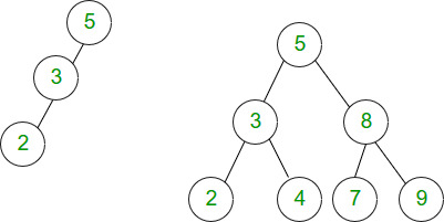
For example, the binary tree shown in figure above with height 2 has 3 nodes:

Minimum Number of nodes = (h+1) = (2 + 1) = 3

Maximum Number of nodes = (2^(h+1) - 1) = 2^(2+1) - 1 = 2^3 - 1 = 8 - 1 = 7

Now its time to calculating minimum and maximum height from the number of nodes:

Calculating Minimum and Maximum height from the Number of Nodes

If there are n nodes in a binary search tree, maximum height of the binary search tree is n-1 and minimum height is ceil(log2(n)+1).

Minimum Height with n Nodes:

• The minimum height with 'n' nodes is achieved in a perfectly balanced binary tree.
• In a balanced binary tree, the number of nodes is distributed evenly among the levels, minimizing the height.
• Therefore, the minimum height with n nodes is given by: ceil[log2(n + 1) -1].

The minimum height is achieved with the maximum number of node (perfectly balanced tree)
From the Maximum number nodes with a height h =>
n = 2^(h+1) -1
n+1 = 2^(h+1)
Taking log both sides
log2(n+1) = log2*2^(h+1)
log2(n+1) = h+1
h = [log2(n+1) - 1]

Maximum Height with n Nodes:

• The maximum height with 'n' nodes is achieved in a completely unbalanced binary tree.
• In an unbalanced binary tree, each node only has one child, leading to a linear structure.
• Therefore, the maximum height with 'n' nodes is 'n - 1'.

As we know that maximum height is achieved by minimum number of nodes:
So,
Using Minimum number of nodes with heigh h formula
n = h + 1
h = n - 1

Traversal:

• Traversal involves visiting each node in the tree in a specific order.
• Common traversal method include:
  → In-order (Left, Root, Right)
  → Pre-order (Root, Left, Right)
  → Post-order (Left, Right, Root)

3 Representation of Binary Tree

A binary tree can be represented using linked list and also using an array.

Array Representation:

The binary tree can be represented using an array of size 2n+1 if the depth of binary tree is n. If the parent element is at the index p, Then the left child will be stored in the index (2p) + 1, and the right child will be stored in the index (2p) + 2.

Root Index:

• The root of the binary tree is stored at index 0 of the array.

Parent-Child Relationship:

• For any node at index i:
  • Its left child is at index 2 * i + 1.
  • Its right child is at index 2 * i + 2.
  • If a node doesn't have a left or right child, the corresponding index in the array will be empty or contain a sentinel value (such as null or -1), depending on the implementation.

Finding Parent Location from Child Node:

• For Left Child (index i): The parent node is at index (i - 1)/2.
• For Right Child (index i): The parent node is at index (i - 2)/2.

Example:

          1
        /   \
       2     3
      / \   / \
     4   5 6   7

[1, 2, 3, 4, 5, 6, 7]

1. For the left child (index 4):
   1. Node 4 is at index 3.
   2. Parent index would be at = (3 - 1)/2 = 2/2 = 1.
   3. So, the parent node of node 4 is at index 1, which is 2.
2. For the right child (index 5):
   1. Node 5 is at index 4.
   2. Parent index would be at = (4 - 2)/2 = 2/2 = 1.
   3. So, the parent node of node 5 is at index 1, which is node 2.

Code:

Converting a Binary Tree to an Array:

Let's consider the following binary tree as an example:

        A
       / \
      B   C
     / \
    D   E

The array representation would be [1, 2, 3, 4, 5]. The root is at index 0, and the left and right children follow the defined relationship.

For example, consider the following binary tree:

       1
     /   \
    2     3
   / \   / \
  4   5 6   7

Its array representation would be [1, 2, 3, 4, 5, 6, 7].

Here's how the indices map to the tree:

• Index 0: Root (1)
• Index 1: Left child of root (2)
• Index 2: Right child of root (3)
• Index 3: Left child of node 2 (4)
• Index 4: Right child of node 2 (5)
• Index 5: Left child of node 3 (6)
• Index 6: Right child of node 3 (7)

Linked List Representation

Representation a binary tree using linked list involves creating nodes that contain information about the data at each node, as well as pointers to the left and right children. This creates a structure similar to the linked list where each node points to its children. 

#include <iostream>

// Define the structure for a binary tree node with structure
struct TreeNode {
    int data;
    TreeNode* left;
    TreeNode* right;

    // Constructor to initialize the node
    TreeNode(int value) : data(value), left(nullptr), right(nullptr) {}
};

or

// Define the structure for a binary tree node with class
class TreeNode {
public:
    int data;
    TreeNode* left;
    TreeNode* right;

    // Constructor
    TreeNode(int value) : data(value), left(nullptr), right(nullptr) {}
};


// Function to perform an in-order traversal of the binary tree
void inorderTraversal(TreeNode* root) {
    if (root != nullptr) {
        inorderTraversal(root->left);
        std::cout << root->data << " ";
        inorderTraversal(root->right);
    }
}

int main() {
    // Creating a sample binary tree
    TreeNode* root = new TreeNode(1);
    root->left = new TreeNode(2);
    root->right = new TreeNode(3);
    root->left->left = new TreeNode(4);
    root->left->right = new TreeNode(5);

    // Performing in-order traversal
    std::cout << "In-order Traversal: ";
    inorderTraversal(root);
    std::cout << std::endl;

    // Additional operations can be added here...

    // Clean up memory by deleting the nodes
    delete root->left->left;
    delete root->left->right;
    delete root->left;
    delete root->right;
    delete root;

    return 0;
}

4 Operations on Binary Trees

1. Insertion:

Inserting a new node into a binary tree involves finding the appropriate position based on the value to be inserted.

Algorithm:

• Start from the root.
• If the value is less than the current node's value, move to the left subtree; otherwise, move to the right subtree.
• Repeat until an empty spot is found, then insert the new node.

Code Implementation:

void insert(TreeNode*& root, int value) {
    if (root == nullptr) {
        root = new TreeNode(value);
    } else if (value < root->data) {
        insert(root->left, value);
    } else {
        insert(root->right, value);
    }
}

2. Deletion:

Deleting a node from a binary tree requires handling three cases:

a node with no children, a node with one child, and a node with two children.

Algorithm:

• If the node to be deleted has no children, simply remove it.
• If the node has one child, replace the node with its child.
• If the node has two children, finds its in-order successor (or predecessor), replace the node's value, and recursively delete the successor.

Implementation:

3. Traversal:

Traversal is the process of visiting nodes in a specific order. Common traversal methods include:

1. In-order Traversal: Visit the left subtree, the current node, and then the right subtree.
2. Pre-order Traversal: Visit the current node, the left subtree, and then the right subtree.
3. Post-order Traversal: Visit the left subtree, the right subtree, and then the current node.

Implementation:

void inorderTraversal(TreeNode* root) {
    if (root != nullptr) {
        inorderTraversal(root->left);
        // Process or print the current node's data.
        inorderTraversal(root->right);
    }
}

void preorderTraversal(TreeNode* root) {
    if (root != nullptr) {
        // Process or print the current node's data.
        preorderTraversal(root->left);
        preorderTraversal(root->right);
    }
}

void postorderTraversal(TreeNode* root) {
    if (root != nullptr) {
        postorderTraversal(root->left);
        postorderTraversal(root->right);
        // Process or print the current node's data.
    }
}

4. Searching

Searching for a value in a binary tree involves traversing the tree based on the comparison of the value with each node.

Algorithm:

• Start from the root.
• If the value is equal to the current node's value, return the node.
• If the value is less, move to the left subtree; otherwise, move to the right subtree.
• Repeat until the value is found or a leaf node is reached.

Implementation:

bool search(TreeNode* root, int value) {
    if (root == nullptr) {
        return false;
    }
    if (root->data == value) {
        return true;
    } else if (value < root->data) {
        return search(root->left, value);
    } else {
        return search(root->right, value);
    }
}

5 Types of Binary Tree

Types of Binary Tree based on the number of children:

1. Full Binary Tree | Strict Binary Tree

A Binary Tree is a full binary tree if every node has 0 or 2 children. It is also known as a proper binary tree. Means in it each node has either zero or two children, but never one.

Example:

        1
       / \
      2   3
     / \
    4   5

2. Degenerate (or pathological) tree

A Tree where every internal node has one child. Such trees are performance-wise same as linked list. A degenerate tree is a tree having a single child either left or right.

3. Skewed Binary Tree

A skewed binary tree is a pathological/degenerate tree in which the tree is either dominated by the left nodes or the right nodes. Thus, there are two types of skewed binary tree: left-skewed binary and right-skewed binary tree.

Types of Binary Tree on the basis of the completion of levels:

• Full Binary Tree
• Complete Binary Tree
• Perfect Binary Tree
• Degenerate Binary Tree
• Balanced Binary Tree

1. Full Binary Trees (Strict || Proper Binary Tree):

A full binary tree is a binary tree in which each node has either zero or two children, but never one. It maintains a consistent structure, ensuring that each level is filled from left to right.

Characteristics:

• Each node has either 0 or 2 children.
• All leaf nodes are at the same level.
• Maintains a regular and balanced structure.

Example:

        1
       / \
      2   3
     / \
    4   5

2. Complete Binary Trees:

A complete binary tree is a binary tree in which all levels, except possibly the last, are completely filled, and all nodes are as left as possible. The last level is filled from left to right.

Characteristics:

• All levels are filled, except possibly the last.
• Nodes are filled from left to right 

      1
    /   \
   2     3
  / \   /
 4   5 6

3. Perfect Binary Tree:

• In a perfect binary tree, all interior nodes have two children, and all leaf nodes are at the same level.
• The number of nodes at each level doubles as you move down the tree.

      1
    /   \
   2     3
  / \   / \
 4   5 6   7

4. Degenerate Binary Tree:

• A degenerate tree is a binary tree where each parent node has only one child.
• Degenerate trees are essentially linked lists in the shape of a tree.

      1
       \
        2
         \
          3
           \
            4

5. Balanced Binary Tree:

• A balanced binary tree is a binary tree in which the height of the left and right subtrees of any node differ by at most one.
• AVL trees and Red-Black trees are examples of balanced binary trees.
• Balancing is maintained through rotations during insertion and deletion operations.
• Operations like insertion, deletion, and searching have a time complexity of O(log n) in balanced trees.

      2
    /   \
   1     3
  / \   / \
 0   0 0   0

6 Complexity Analysis and Performance Considerations of Binary Trees

Binary trees are fundamental data structures with various operations, each with its own time and space complexity.

6.1 Time Complexity:

1. Search (Average Case): O(log n)
   1. In a balanced binary tree (such as a binary search tree), the time complexity for searching an element is logarithmic. This is because at each step, the search space is reduced by half.
   2. However, in the worst-case scenario (unbalanced tree), the time complexity can degrade to O(n), where n is the number of nodes in the tree.
2. Insertion (Average Case): O(log n)
   1. Similar to searching, insertion in a balanced binary tree has logarithmic time complexity on average.
   2. In the worst-case scenario (unbalanced tree), insertion can also degrade to O(n).
3. Deletion (Average Case): O(log n)
   1. Deletion in a balanced binary tree also has logarithmic time complexity on average.
   2. However, in the worst-case scenario (unbalanced tree), deletion can degrade to O(n).
4. Traversal (Preorder, Inorder, Postorder): O(n)
   1. Traversal of a binary tree requires visiting every node once.
   2. Hence, the time complexity of traversal algorithms is linear, O(n), where n is the number of nodes in the tree.

6.2 Space Complexity:

• Storage: O(n)
  • Binary trees consume space proportional to the number of nodes in the tree.
  • Each node in the tree requires memory for storing data and pointers to its left and right children.

6.3 Performance Considerations:

1. Balancing:
   1. Unbalanced binary trees can lead to degraded performance. It's essential to ensure that binary trees remain balanced to maintain optimal time complexity for operations like search, insertion, and deletion.
   2. Techniques such as AVL trees and Red-Black trees are used to ensure balancing.

7 Tree Traversal Techniques

A Tree Data Structure can be traversed in following ways:

1. Depth First Search (DFS)
   1. Inorder Traversal
   2. Preorder Traversal
   3. Postorder Traversal
2. Breadth First Search (BFS) || Level Order Traversal

7.1 Depth First Search (DFS):

DFS (Depth-first search) is a technique used for traversing trees or graphs. Here backtracking is used for traversal. In this traversal first, the deepest node is visited and then backtracks to its parent node if no sibling of that node exists

It checks all nodes from leftmost path from the root to the leaf, then jumps up and check right node and so on.

• It uses a stack to keep track of the next location to visit.

Consider the binary tree:

       1
     /   \
    2     3
   / \   / \
  4   5 6   7

DFS traversal of this tree would visit nodes in the order: 1 -> 2 -> 4 -> 5 -> 3 -> 6 -> 7

Process:

1. Start with the root node.
2. Process the current node.
3. Recursively visit the left subtree.
4. Recursively visit the right subtree.
5. Repeat until all nodes are visited.

There are three main ways to apply Depth First Search to a tree.

They are as follows:

1 Preorder Traversal:

We start from the root node and search the tree vertically (top to bottom), traversing from left to right. The order of visits is ROOT-LEFT-RIGHT.

Algorithm:

1. Visit the current node.
2. Recursively traverse the left subtree.
3. Recursively traverse the right subtree.

Example:

       1
     /   \
    2     3
   / \   / \
  4   5 6   7

Pre-order traversal of this tree would visit nodes in the order: 1 -> 2 -> 4 -> 5 -> 3 -> 6 -> 7

Implementation in C++:

#include <iostream>

using namespace std;

// Binary Tree Node
struct TreeNode {
    int data;
    TreeNode* left;
    TreeNode* right;
    
    TreeNode(int val) : data(val), left(nullptr), right(nullptr) {}
};

// Pre-order Traversal Function
void preorderTraversal(TreeNode* root) {
    if (root == nullptr) return;

    // Visit current node
    cout << root->data << " ";

    // Recursively traverse left subtree
    preorderTraversal(root->left);

    // Recursively traverse right subtree
    preorderTraversal(root->right);
}

int main() {
    // Construct the binary tree
    TreeNode* root = new TreeNode(1);
    root->left = new TreeNode(2);
    root->right = new TreeNode(3);
    root->left->left = new TreeNode(4);
    root->left->right = new TreeNode(5);
    root->right->left = new TreeNode(6);
    root->right->right = new TreeNode(7);

    // Perform pre-order traversal
    cout << "Pre-order Traversal: ";
    preorderTraversal(root);
    cout << endl;

    return 0;
}

Output:

Pre-order Traversal: 1 2 4 5 3 6 7 

2 In-order Traversal

Start from the leftmost node and move to the right nodes traversing from top to bottom. The order of visits is LEFT-ROOT-RIGHT.

Algorithm:

1. Recursively traverse the left subtree.
2. Visit the current node.
3. Recursively traverse the right subtree.

Example:

Consider the following binary tree:

       1
     /   \
    2     3
   / \   / \
  4   5 6   7

In-order traversal of this tree would visit nodes in the order: 4 -> 2 -> 5 -> 1 -> 6 -> 3 -> 7

Implementation in C++:

#include <iostream>

using namespace std;

// Binary Tree Node
struct TreeNode {
    int data;
    TreeNode* left;
    TreeNode* right;
    
    TreeNode(int val) : data(val), left(nullptr), right(nullptr) {}
};

// In-order Traversal Function
void inorderTraversal(TreeNode* root) {
    if (root == nullptr) return;

    // Recursively traverse left subtree
    inorderTraversal(root->left);

    // Visit current node
    cout << root->data << " ";

    // Recursively traverse right subtree
    inorderTraversal(root->right);
}

int main() {
    // Construct the binary tree
    TreeNode* root = new TreeNode(1);
    root->left = new TreeNode(2);
    root->right = new TreeNode(3);
    root->left->left = new TreeNode(4);
    root->left->right = new TreeNode(5);
    root->right->left = new TreeNode(6);
    root->right->right = new TreeNode(7);

    // Perform in-order traversal
    cout << "In-order Traversal: ";
    inorderTraversal(root);
    cout << endl;

    return 0;
}

Output:

In-order Traversal: 4 2 5 1 6 3 7

3 Post order Traversal

Start from the leftmost node and move to the right nodes, traversing from bottom to top. The order of visits is LEFT-RIGHT-ROOT.

Algorithm:

1. Recursively traverse the left subtree.
2. Recursively traverse the right subtree.
3. Visit the current node.

Example:

Consider the following binary tree:

       1
     /   \
    2     3
   / \   / \
  4   5 6   7

Post-order traversal of this tree would visit nodes in the order: 4 -> 5 -> 2 -> 6 -> 7 -> 3 -> 1

Implementation in C++:

#include <iostream>

using namespace std;

// Binary Tree Node
struct TreeNode {
    int data;
    TreeNode* left;
    TreeNode* right;
    
    TreeNode(int val) : data(val), left(nullptr), right(nullptr) {}
};

// Post-order Traversal Function
void postorderTraversal(TreeNode* root) {
    if (root == nullptr) return;

    // Recursively traverse left subtree
    postorderTraversal(root->left);

    // Recursively traverse right subtree
    postorderTraversal(root->right);

    // Visit current node
    cout << root->data << " ";
}

int main() {
    // Construct the binary tree
    TreeNode* root = new TreeNode(1);
    root->left = new TreeNode(2);
    root->right = new TreeNode(3);
    root->left->left = new TreeNode(4);
    root->left->right = new TreeNode(5);
    root->right->left = new TreeNode(6);
    root->right->right = new TreeNode(7);

    // Perform post-order traversal
    cout << "Post-order Traversal: ";
    postorderTraversal(root);
    cout << endl;

    return 0;
}

Output:

Post-order Traversal: 4 5 2 6 7 3 1

7.2 Breadth-first Search

In Breadth First Search (BFS), the key is that it is a level-based, or row-based movement. At each level or row, the nodes of a tree are visited/traversed horizontally from left to right or right to left.

It explores all the vertices level by level. It starts at the root node or an arbitrary node and visits all the nodes at the same level before moving on to the next level.

Consider the following binary tree:

        1
      /   \
     2     3
    / \   / \
   4   5 6   7

Starting from the root node 1, we will perform a Breadth-First Search traversal to explore all the nodes level by level.

Step-by-Step Illustration:

1. Level 1 (Root Node):
   1. Enqueue node 1 into the queue.
   2. Dequeue node 1 from the queue and process it.
   3. Enqueue its children 2 and 3.
2. Level 2:
   1. Dequeue node 2 from the queue and process it.
   2. Enqueue its children 4 and 5.
   3. Dequeue node 3 from the queue and process it.
   4. Enqueue its children 6 and 7.
3. Level 3:
   1. Dequeue node 4 from the queue and process it.
   2. Dequeue node 5 from the queue and process it.
   3. Dequeue node 6 from the queue and process it.
   4. Dequeue node 7 from the queue and process it.

Visualization:

        1            <-- Level 1
      /   \
     2     3         <-- Level 2
    / \   / \
   4   5 6   7       <-- Level 3

Final Traversal Order:

Breadth-First Search Traversal: 1 2 3 4 5 6 7

Code Implementation in C++:

#include <iostream>
#include <queue>

using namespace std;

struct TreeNode {
    int data;
    TreeNode* left;
    TreeNode* right;

    TreeNode(int val) : data(val), left(nullptr), right(nullptr) {}
};

void breadthFirstSearch(TreeNode* root) {
    if (root == nullptr) return;

    queue<TreeNode*> q;
    q.push(root);

    while (!q.empty()) {
        TreeNode* current = q.front();
        q.pop();

        cout << current->data << " ";

        if (current->left != nullptr) q.push(current->left);
        if (current->right != nullptr) q.push(current->right);
    }
}

int main() {
    TreeNode* root = new TreeNode(1);
    root->left = new TreeNode(2);
    root->right = new TreeNode(3);
    root->left->left = new TreeNode(4);
    root->left->right = new TreeNode(5);
    root->right->left = new TreeNode(6);
    root->right->right = new TreeNode(7);

    cout << "Breadth-First Search Traversal: ";
    breadthFirstSearch(root);
    cout << endl;

    return 0;
}

8 Difference between BFS and DFS

1 Traversal Order:

• BFS (Breadth-First Search):
  • Traverses the tree level by level, starting from the root node and visiting all nodes at each level before moving to the next level.
  • Visits nodes in increasing order of depth from the root.
  • Emphasizes horizontal traversal, exploring sibling nodes before moving deeper into the tree.
• DFS (Depth-First Search):
  • Traverses the tree depth by depth, exploring as far as possible along each branch before backtracking.
  • Visits nodes in a vertical manner, diving deep into the tree before exploring sibling nodes.
  • Emphasizes deep traversal, exploring the entire depth of each subtree before moving to the next subtree.

2. Data Structure:

• BFS:
  • Utilizes a queue data structure to keep track of the nodes to be visited next.
  • Enqueues nodes as they are discovered and dequeues nodes for processing in the order they were enqueued.
  • Guarantees that nodes are visited in the order of their depth from the root.
• DFS:
  • Can be implemented using either recursion or a stack data structure (implicitly via the call stack in recursive implementations).
  • Visits nodes depth-first, pushing nodes onto the stack as they are discovered and popping nodes for processing in the reverse order of discovery.
  • Does not guarantee a specific order of traversal; the order depends on the implementation (e.g., pre-order, in-order, post-order).

3. Memory Usage:

• BFS:
  • Typically requires more memory compared to DFS due to the need to maintain a queue data structure.
  • Enqueues all child nodes of a parent node before dequeuing and processing them.
• DFS:
  • Generally uses less memory compared to BFS, especially in recursive implementations.
  • Only requires enough memory to store the call stack when using recursion, or a small stack for iterative implementations.

4. Applications:

• BFS:
  • Well-suited for finding the shortest path between two nodes in an unweighted graph or tree.
  • Useful for applications requiring level order traversal, such as serialization and deserialization of tree structures.
• DFS:
  • Suitable for applications requiring deep traversal, such as backtracking, cycle detection, and topological sorting.
  • Often used in tasks like tree traversal, expression tree evaluation, and memory management in garbage collection algorithms.