Those who cannot remember the past are condemned to repeat it.. says the ~DP.

Try all possible ways… says the ~Recursion.

Dynamic Programming (DP) is a powerful algorithmic technique used for solving optimization problems. It is particularly useful when a problem can be broken down into overlapping subproblems that can be solved independently, and the results of these subproblems can be reused to find the solution to the original problem. Dynamic programming helps in reducing the time complexity by avoiding the re-computation of subproblems, which is a significant improvement over naive recursion.

Dynamic Programming = Recursion + Storage.

When to Use Dynamic Programming

Dynamic Programming is used when:

1. Optimal Substructure: A problem exhibits optimal substructure if the solution to the problem can be constructed from solutions to its subproblems.
   • If asked about Optimal answer.
2. Overlapping Subproblems: A problem exhibits overlapping subproblems if the problem can be broken down into smaller subproblems which are reused multiple times.
   • If there are two function calls.

Dynamic Programming vs Divide and Conquer

• Divide and Conquer: Divides the problem into non-overlapping subproblems, solves them independently, and combines their solutions.
• Dynamic Programming: Divides the problem into overlapping subproblems, solves each subproblem only once, and reuses the solution when needed.

Memory-Time Tradeoff

Dynamic Programming (DP) is a powerful optimization technique, but it often requires storing solutions to subproblems, leading to a tradeoff between memory usage and time efficiency. The essence of this tradeoff is simple: by using more memory to store precomputed results of subproblems, we can save time by avoiding redundant calculations. 

DP improves the time complexity by avoiding re-computation of the same subproblems, typically reducing exponential time complexities to polynomial time complexities.

Types of Dynamic Approach

1️⃣ Top-Down (Memoization) Approach

In the Top-Down approach, you solve a problem by breaking it into smaller subproblems recursively. While doing so, you store the results of each subproblem in a memoization table (usually a dictionary or an array). When a subproblem arises multiple times, you can look up the result in the memoization table instead of recalculating it.

Characteristics:

• Recursion is used.
• Memoization (caching) is applied to store the results of subproblems.
• It's easier to implement if you're comfortable with recursion.
• It starts from top (required answer which is n) goes to the base case and then come back that's why it is top down.

2️⃣ Bottom-Up (Tabulation) Approach

In the Bottom-Up approach, you solve the problem iteratively. Instead of starting from the main problem and breaking it down, you start by solving the smallest subproblems first and gradually build up solutions to larger subproblems using a DP table.

Characteristics:

• Iteration is used.
• Tabulation (a table) is built from the ground up.
• Generally more space-efficient than the top-down approach because you don't have the overhead of recursion.
• Here we start from the base case, and goes up to the required answer (top).

Why Dynamic Programming (DP) is Used in DSA

Dynamic Programming (DP) is a critical technique in algorithm design because it offers an efficient solution to problems that exhibit overlapping subproblems and optimal substructure. DP is used to improve the performance of algorithms by avoiding redundant computations and efficiently solving problems that would otherwise take exponential time using straightforward recursion or brute-force approaches.

Here are the primary reasons why DP is used in Data Structures and Algorithms (DSA):

1. Solves Overlapping Subproblems

Many problems involve solving the same subproblems repeatedly. In a brute-force recursive approach, these subproblems are recalculated multiple times, which leads to inefficiency. DP stores the results of these subproblems (either in a table or cache), so they are computed only once.

Example:

In the Fibonacci sequence, without DP, you would re-compute smaller Fibonacci numbers multiple times.

Brute-force Recursive Fibonacci:

int fib(int n) {
    if (n <= 1) return n;
    return fib(n - 1) + fib(n - 2);
}

This approach will calculate the same Fibonacci numbers multiple times, leading to a time complexity of O(2^n).

Recursive Call Tree:

Let's take n = 5 as an example and draw the recursive call tree:

fib(5)
├── fib(4)
│   ├── fib(3)
│   │   ├── fib(2)
│   │   │   ├── fib(1) → returns 1
│   │   │   └── fib(0) → returns 0
│   │   └── fib(1) → returns 1
│   └── fib(2)
│       ├── fib(1) → returns 1
│       └── fib(0) → returns 0
└── fib(3)
    ├── fib(2)
    │   ├── fib(1) → returns 1
    │   └── fib(0) → returns 0
    └── fib(1) → returns 1

• Notice that many subproblems are recalculated multiple times. For example, fib(2) and fib(1) are computed several times.
  • We solved some problem before and we again encountered same problem again, that is called as overlapping sub problems. Whenever we end up solving same problem again and again, then we call it overlapping sub problems.
• The tree grows exponentially, with each fib(n) call resulting in two more calls, leading to an explosion in the number of function calls.

Counting the Number of Calls:

• For each n , the function makes 2 recursive calls: fib(n - 1) and fib(n - 2).
• Each of these recursive calls leads to further calls, creating a binary tree of recursive calls.
• The depth of this tree is n , and at each level, the number of function calls doubles. This results in 2^n nodes (function calls) in the tree.

Optimized DP (with memoization):

• Here we tend to store the value of sub problems. so that we don't need to recompute the recurring problems again and again.

int fib(int n, vector<int>& memo) {
	// Base case: return n if n is 0 or 1
    if (n <= 1) return n;
    
    // If the value is already calculated, return it
    if (memo[n] != -1) return memo[n];  // Return memoized result
    
    // calculate the value and store it in memo array
    memo[n] = fib(n - 1, memo) + fib(n - 2, memo);
    return memo[n];
}

int main() {
    int n = 10; // Fibonacci number to find
    vector<int> memo(n + 1, -1);  // Initialize memo array with -1.
    
    // Output the nth Fibonacci number
    cout << fib(n, memo) << endl;
    return 0;
}

This reduces the time complexity to O(n) by using memoization or tabulation, as each subproblem is solved only once. These methods avoid recalculating the same Fibonacci number multiple times by storing intermediate results.

Complexity Analysis:

• Time Complexity:O(N) Overlapping subproblems return answers in constant time O(1). Therefore, only 'n' new subproblems are solved, resulting in O(N) complexity.
• Space Complexity:O(N) Using recursion stack space and an array, the total space complexity is O(N) + O(N) ≈ O(N).

Steps to Memoize a Recursive Solution:

1. Create a array | vector maybe of name memo or whatever, of size n + 1, initialized to -1.
2. Check if the answer is already calculated by looking at memo[n] !=-1. If yes return the value.
3. If not, compute the value and store it in the memo array before returning.

Tabulation (Bottom Up) Approach:

Tabulation, also known as "bottom-up" dynamic programming, involves solving the problem by iteratively solving all possible sub-problems, starting from the base cases and building up to the solution of the main problem. The results of sub-problems are stored in a table, and each entry in the table is filled based on previously computed entries.

Steps to Convert Recursive Solution to Tabulation:

1. Declare a dp[] array of size n+1, you can give the array name you want, I give it dp name to distinguish it from memoization memo array.
2. Initialize base condition values, i.e, i = 0 and i = 1 of the dp array as 0 and 1 respectively.
3. Use an iterative loop to traverse the array (from index 2 to n) and set each value as dp[i - 1] + dp[i - 2].

#include <bits/stdc++.h>

using namespace std;

int main() {
    int n = 5; // Fibonacci number to find

    // Initialize dp array with size n + 1
    vector<int> dp(n + 1);

    // Base cases
    dp[0] = 0;
    dp[1] = 1;

    // Fill the dp array using the tabulation method
    for (int i = 2; i <= n; i++) {
        dp[i] = dp[i - 1] + dp[i - 2];
    }

    // Output the nth Fibonacci number
    cout << dp[n] << endl;

    return 0;
}

Complexity Analysis:

• Time Complexity:O(N): Running a simple iterative loop results in O(N) complexity.
• Space Complexity:O(N): Using an external array of size n+1, the space complexity is O(N).

Solution: Space Optimization:

The relation dp[i] = dp[i-1] + dp[i-2] shows that only the last two values in the array are needed. By maintaining only two variables (prev and prev2), space can be optimized. This optimization reduces the space complexity from O(N) to O(1) since it eliminates the need for an entire array to store intermediate results.

In each iteration, compute the current Fibonacci number using the values of prev and prev2. Assign the value of prev to prev2 and the value of the current Fibonacci number to prev. This way, the variables are updated for the next iteration. After the loop completes, the variable prev holds the value of the nth Fibonacci number, which is then returned as the result.

#include <bits/stdc++.h>

using namespace std;

int main() {
    int n = 5; // Fibonacci number to find

    // Edge case: if n is 0, the result is 0
    if (n == 0) {
        cout << 0;
        return 0;
    }

    // Edge case: if n is 1, the result is 1
    if (n == 1) {
        cout << 1;
        return 0;
    }

    int prev2 = 0; // Fibonacci number for n-2
    int prev = 1;  // Fibonacci number for n-1

    // Iterate from 2 to n to find the nth Fibonacci number
    for (int i = 2; i <= n; i++) {
        int cur_i = prev2 + prev; // Current Fibonacci number
        prev2 = prev;             // Update prev2 to the previous Fibonacci number
        prev = cur_i;             // Update prev to the current Fibonacci number
    }

    // Print the nth Fibonacci number
    cout << prev;
    return 0;
}

Complexity Analysis:

• Time ComplexityO(N) : We are running a simple iterative loop
• Space ComplexityO(1) : We are not using any extra space

DP Categories

1️⃣ 0/1 Knapsack Type

It is actually a very classic category of Dynamic Programming (DP).

• Each item can be taken once or not at all (Pick, Skip)
• Problems:
  1. 0/1 Knapsack: https://thejat.in/code/knapsack-problem
  2. Painting the walls: https://thejat.in/code/painting-the-walls
  3. Subset Sum Problem: https://thejat.in/code/subset-sum-equals-to-target
     1. Is there a subset whose sum is equal to a given value?
  4. Partition Equal Subset Sum (Equal Sum Partition): https://thejat.in/code/partition-equal-subset-sum
     1. Can the array be split into two subsets with equal sum?
  5. Minimum Subset Sum Problem: 
  6. Partition a set into two subsets with minimum absolute difference: https://thejat.in/code/partition-a-set-into-two-subsets-with-minimum-absolute-sum-difference
  7. Count of Subsets with Given Sum: https://thejat.in/code/count-subsets-with-sum-k
     1. Count how many subsets add up to a specific sum.
  8. Target Sum: https://thejat.in/code/target-sum
     1. Assign + and - to elements to reach a target sum.
  9. Number of Subsets with Given Difference

2️⃣ Unbounded Knapsack Type

• Each item can be taken infinite times
• Problems:
  • Unbounded Knapsack: https://thejat.in/code/knapsack-problem
  • Coin Change (Min no. of ways): https://thejat.in/code/minimum-number-of-coins-to-make-a-target
  • Coin change 2: https://thejat.in/code/coin-change-2
  • Rod Cutting: https://thejat.in/code/rod-cutting-problem
  • Integer Break

3️⃣ Fibonacci Style / Linear DP

• Problems with recurrence like: dp[i] = dp[i - 1] + dp[i - 2]
  • Recurrence based on previous indices
• Problems:
  • Fibonacci
  • Climbing Stairs
  • House Robber
  • Decode Ways
  • Tribonacci

4️⃣ Kadane's Algorithm Type

• Subarray-based maximum/minimum sum problems
• Problems:
  • Maximum Subarray Sum
  • Maximum Product Subarray

5️⃣ Partition DP || Matrix Chain Multiplication (MCM) / Interval DP

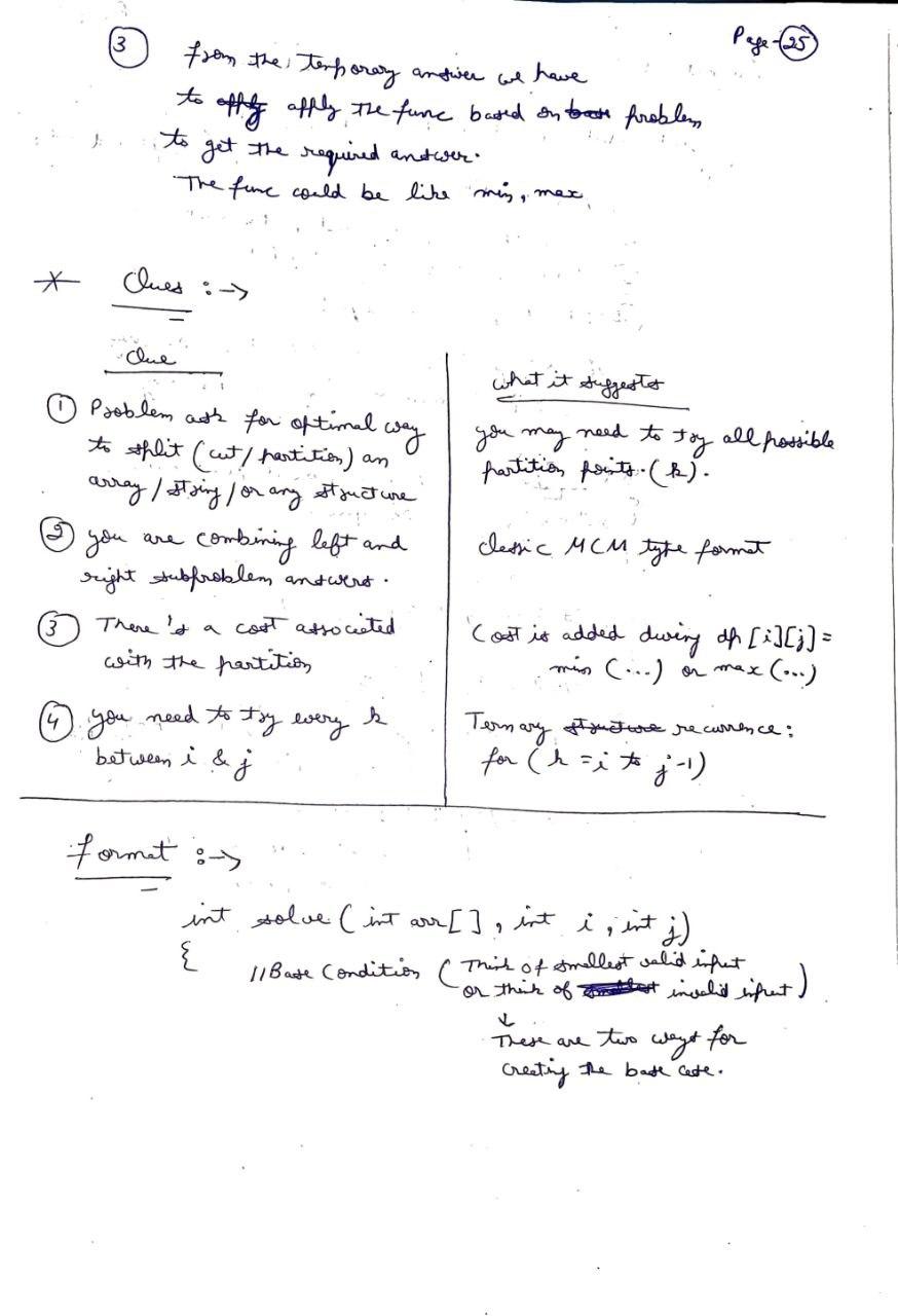
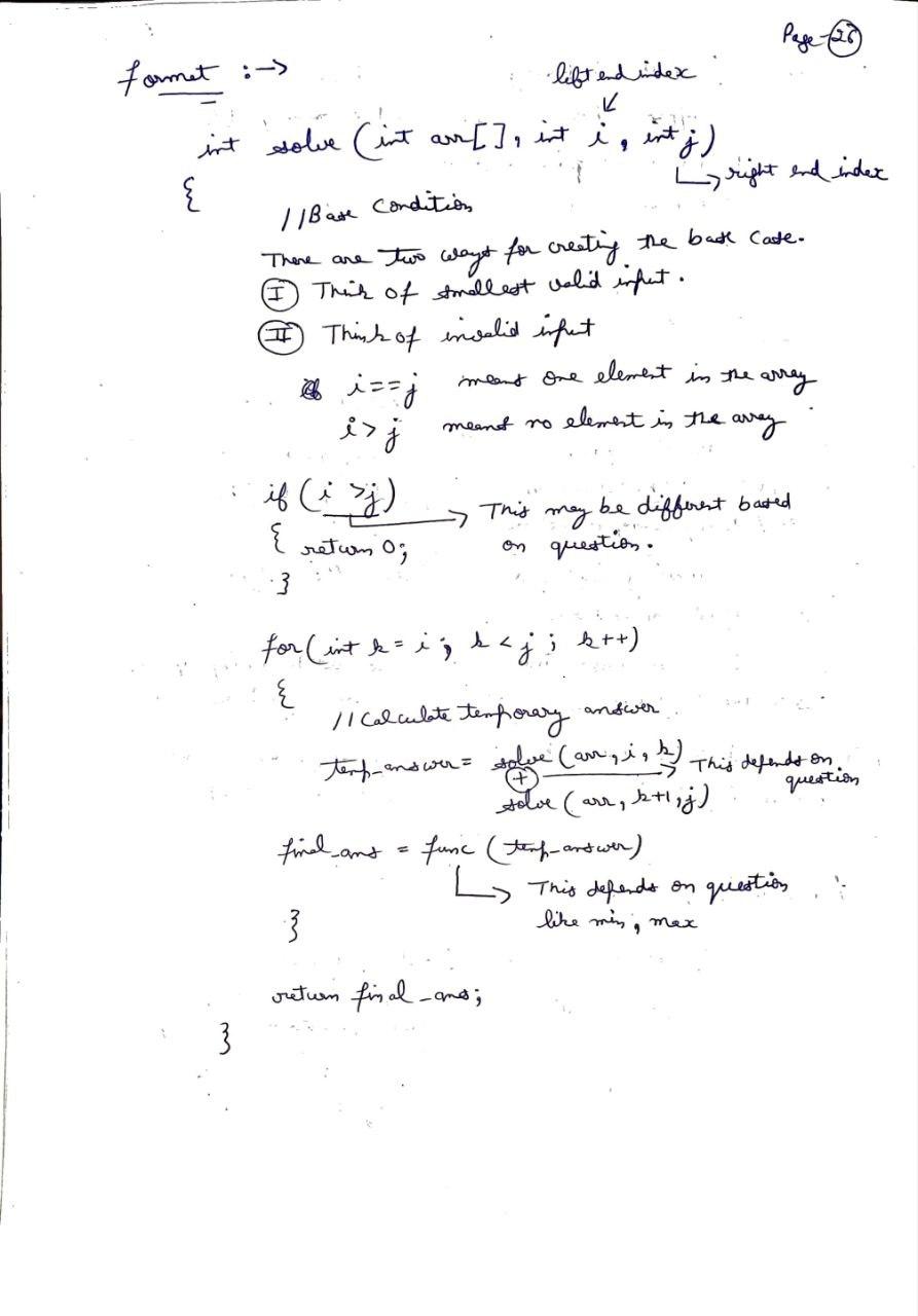
• Partition DP (also known as “MCM-type DP” is a category of dynamic programming problems where you partition the input into segments or subproblems, and computer the answer using choices of partition points (like splitting an array or string at different indices).
• In simple terms: Problems where we try all ways to partition input (string/array) and choose the best by combining solutions from left and right parts.
• DP on ranges or intervals in arrays
• Problems:
  • Matrix Chain Multiplication: https://thejat.in/code/matrix-chain-multiplication
  • Minimum Cost to Cut a Stick: https://thejat.in/code/minimum-cost-to-cut-the-stick
  • Burst Balloons: https://thejat.in/code/burst-balloons
  • Palindrome Partitioning 2
  • Boolean Parenthesization
  •  
  • Scrambled String

6️⃣ DP on Trees

• Use post-order traversal to compute DP from children
• Problems:
  • Diameter of Binary Tree
  • House Robber 3
  • Count Paths with Given Sum

7️⃣ DP on Grids (2D DP)

• DP based on movement in grids or matrices
• Problems:
  • Unique Paths
  • Minimum Path Sum
  • Dungeon Game
  • Cherry Pickup

8️⃣ Digit DP

• Use digit-level states to count numbers satisfying constraints
• Problems:
  • Count numbers less than N with digit sum S
  • Count of numbers with no adjacent same digits

9️⃣ DP on Bitmask

Bitmask DP is used when you need to track a subset of elements efficiently. Each bit in a binary number represents whether an item is included or not — perfect for problems involving permutations, combinations, and states.

• Use a bitmask to represent a subset of visited elements
• Problems:
  • Traveling Salesman Problem
  • Assignments / Job Scheduling
  • Minimum Incompatibility
  • Shortest Path Visiting All Nodes: https://thejat.in/code/shortest-path-visiting-all-nodes

1️⃣0️⃣ DP on Strings

• Often overlaps with subsequence-type problems
• Problems:
  • Edit Distance
  • Interleaving Strings
  • Wildcard / Regex Matching

1️⃣1️⃣ DP with State Compression / Optimization

• Use tricks to reduce time/space
• Problems:
  • Space Optimization (2D→ 1D)
  • Convex Hull Trick
  • Divide and Conquer DP

1️⃣2️⃣ Game Theory DP

• Player take turns; choose optimal moves
• Problems:
  • Predict the Winner
  • Stone Game variants
  • Minimax with DP

1️⃣3️⃣ DP on Subsequences

• Include / Exclude Decisions

1️⃣4️⃣ Longest Common Subsequences (LCS)

1. Longest Common Subsequence: https://thejat.in/code/longest-common-subsequence
2. Print LCS: https://thejat.in/code/print-longest-common-substring-lcs
3. Longest Common Substring: https://thejat.in/code/longest-common-substring
4. Shortest Common Supersequence: https://thejat.in/code/length-of-shortest-common-super-sequence
5. Print SCS: https://thejat.in/code/shortest-common-super-sequence
6. Longest Palindromic Subsequence: https://thejat.in/code/longest-palindromic-subsequence
7. Minimum insertions to make the string palindrome: https://thejat.in/code/minimum-insertions-to-make-string-palindrome
8. Minimum Number of Insertions and Deletions: https://thejat.in/code/minimum-insertions-to-make-string-palindrome
9. Minimum deletions to make strings equal:
10. Minimum insertions or deletions to convert string A to B: https://thejat.in/code/minimum-insertions-or-deletions-to-convert-string-a-to-b
11. Longest Repeating Subsequence
12. Distinct Subsequences: https://thejat.in/code/distinct-subsequences
13. Edit distance: https://thejat.in/code/edit-distance
14. Wildcard matching: https://thejat.in/code/wildcard-matching

1️⃣5️⃣ Longest Increasing Subsequences (LIS)

1. Longest Increasing Subsequence: https://thejat.in/code/longest-increasing-subsequence
2. Print Longest Increasing Subsequence: 
3. Largest Bitonic Subsequence:
4. Number of Longest Increasing Subsequences:
5. Russian dolls:
6.  

1️⃣6️⃣ State Machine DP

You're designing a machine that changes states based on decisions (buy, sell, rest, hold, etc.). The state keeps track of:

• What you’ve done so far
• What your current status is
• What options are available next
• We use DP[state][day] or DP[day][state] to track transitions.

1. Stock Buy/Sell Problems

1️⃣7️⃣ Digit DP

Digit DP is a dynamic programming technique used to count or construct numbers digit-by-digit under constraints, typically from 1 to n.

Have you ever come across a problem that asks:

• How many numbers between 1 and N have all unique digits? or
• How many numbers from 1 to R have a digit sum ≤ K

These are classic Digit DP problems.

What's Digit DP?

Digit DP is a technique used to count or construct numbers digit-by-digit, often when you are given a range like 1 to N and there are constraints on the digits.

When to Use Digit DP?

You should consider Digit DP when:

• Range given [L, R]
• Count the total number of digit which is equal to 3, in each number lies between [L, R]
• Big N (like up to 10^18): Hints you are counting huge numbers. Brute force won't work – you need to build numbers digit by digit.

Types of Problems:

1. Count of integers x in range [0, R] that satisfies some property f(x).

   You're asked:
      “How many integers x exist such that 0 ≤ x ≤ R and f(x) is true?”
   Where:
      R is a large number (e.g., up to 10^18)
      f(x) is some condition applied on digits of x

   Why not Brute Force?

   You can't loop from 0 to R (too slow).

   Instead, you build numbers digit-by-digit using Digit DP and only count those that satisfies f(x).

   Common f(x) Examples:
   
   1. Digits are unique.
   2. Digit sum <= k
   3. Contains even digit only
   4. No two consecutive equal digits
   5. Is divisible by 7

2. Count how many number x exists such that: L ≤ x ≤ R and f(x) returns true.

   where:

   f(x) is a binary function – it returns either true or false for a number x.

   Examples:
   
   1. f(x): "x has all unique digits"
   2. f(x): "digit sum of x <= 10"
   3. f(x): "x contains no two consecutive equal digits"

   You can't brute force all numbers L to R (might be up to 10^18), instead you define a function like this:

   int solve(N) = count of numbers in [0, N] where f(x) is true
   

   Then the final answer is:

   solve(R) - solve(L - 1)

   This trick automatically handles the range.

Others:

• Minimum cost to cut a stick: https://thejat.in/code/minimum-cost-to-cut-the-stick

Tips & Tricks

1️⃣ Use vector<vector<int>> instead of vector<vector<bool>> in Memoization

For instance if we use:

if (dp[index][target] != false) {
    return dp[index][target];
}

Here we are checking:

• If dp[index][target] != false, then memoization
• But false can mean two things:
  • Either “We solved and answer is false”
  • Or “We have never solved this state”

And if we use:

if (dp[index][target] != -1) {
    return dp[index][target];
}

• We only solve a state once.
• -1 means unsolved and 0/1 means already solved.
• So perfect memoization happens.

Thus in bool version we cannot distinguish between not solved and solved with false.

• Wrong answer might be returned.
• Or recursive calls happen again and again for the same (index, target).
• Hence, huge extra work, which ultimately gives TLE.

If we want to use bool version, we would need a way to keep track of visited or not.

For example:- We can use the visited array.

class Solution{   
public:
    bool solve(vector<int>& arr, int index, int target, vector<vector<bool>>& dp, vector<vector<bool>>& visited){
        if (target == 0) return true;
        if (target < 0 || index == arr.size()) return false;

        if (visited[index][target]) return dp[index][target];

        visited[index][target] = true; // mark as visited

        bool takeIt = false;
        if (arr[index] <= target) {
            takeIt = solve(arr, index + 1, target - arr[index], dp, visited);
        }

        bool skipIt = solve(arr, index + 1, target, dp, visited);

        return dp[index][target] = takeIt || skipIt;
    }

    bool isSubsetSum(vector<int> arr, int target){
        int n = arr.size();
        vector<vector<bool>> dp(n+1, vector<bool>(target+1, false));
        vector<vector<bool>> visited(n+1, vector<bool>(target+1, false));

        return solve(arr, 0, target, dp, visited);
    }
};

• dp[index][target] stores answer
• visited[index][target] stores whether the state is calculated.
• It will not give TLE even with bool.

References

1. https://www.hackerearth.com/practice/algorithms/dynamic-programming/introduction-to-dynamic-programming-1/tutorial/